Diffusion MRI From Quantitative Measurement to In-vivo Neuroanatomy
Chapter 1, Introduction
Diffusion 原理,Free Diffusion
Fick’s first law:
\[J=-D\nabla C\]J是net particle flux,C是particle concentration,D is diffusion coefficient (defined by size of diffusion molecules, temperature, microstructural features of the environment)
diffusion 来源:仅仅是 collisions between atoms or molecules。不管在平衡态还是非平衡态,微观上都有运动。
\[<x^2>=2D\Delta\]x 是diffusion distance,时间是$\Delta$。
MR signal attenuation,用来测量MR的relaxation。
\[E(q)=S(q)/S(0), \quad q=\gamma \delta G\]eliminates the effect of relaxation。
\[E(q)=\int\rho(x_1)\int P(x_1,x_2,\Delta)e^{-iq(x_2-x_1)}dx_1dx_2\]Diffusion propogator (Green’s function): $P(x_1,x_2,\Delta)$,表示particle 一开始在$x_1$,$\Delta$之后,在$x_2$的概率。
$\rho(x_1)$:代表了在$x_1$处找到一个particle 的概率。
\[lim_{t->\infin}P(x_1,x_2,t)=\rho(x_1)\]因为当 $t->\infin$时,一个particle到空间任何一个位置都有相同的概率,这种情况就跟在$x_1$处有一个particle 一样。
Free Diffusion:$E(q)=e^{-q^2D\Delta}$, 考虑pulse duration后,$E(q)=e^{-q^2D\Delta-\delta/3}=e^{-bD}$,
b-value:其中的$b=q^2(\Delta-\delta/3)$
上述方法可以用来描述free, anisotropic diffusion in the principal frame of reference
我们不希望预设任何数学模型,只希望获得local propogator来measure microstructural features。但是low resolution和inability to obtain spin density阻碍了local propogator的获得,因此我们ensemble average来简化问题。
\[E(q)=\int\overline{P}(x,\Delta)e^{-iqx}dx\\\overline{P}(x,\Delta)=\int\rho(x_1)P(x_1,x_1+\Delta x,t)dx_1\]可以看到$E(q)$和$x$之间通过 Fourier Transform联系起来,q-space imaging, Diffusion Spectrum Imaging。
Diffusion in Neural Tissue (影响free diffusion 的因素)
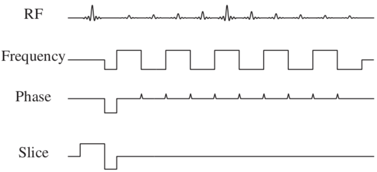
Chapter 2, Pulse Sequence for Diffusion-Weighted MRI
Adding Diffusion Weighting to Pulse Sequence
generalized b-value definition: $b=\int |k_x(t)|^2+|k_y(t)|^2+|k_z(t)|^2 dt$,$k_x(t)=\gamma\int G_x(t)dt$ position on k-space
Two sources of error in DWI: eddy currents, gradient nonlinearity
eddy currents 原理:gradient coils 会产生magnetic fields ,进而在超导线圈周围的液氦中产生感生电场,也就是eddy current。主要由gradient slewing 产生,梯形gradient的上升支和下降支可以相互抵消。
Bulk Motion Sensitivity
Two sources of bulk motion: head movement,cardiac pulsation
different shots will lead to different motion, so DWI are generally limited to single-shot, and the motion remains constant.
一般为了减少采集时间,默认为中心对称的k-space上,我们会进行asymmetric sampling,其中一半可以减少采样数。但是如果由于head rotation,对称假设不再满足,进而产生artifact
navigator correction
Single-shot EPI (SS-EPI)
- geometric warping from field inhomogeneities
- geometric warping from gradient-induced eddy currents
- Intra-voxel dephasing effects on image resolution
Chapter 3, Diffusion Acquisition: Pushing the Boundaries
Chapter 4, Geometric Distortions in Diffusion MRI
dMRI 图像相比与structural image 模糊的原因主要由acquisition 序列EPI造成
EPI对 off-resonance field (实际的field 和我们想要的field的差别)比较敏感。
dMRI中的off-resonance field 由 head 和 after effects of switching the gradients 造成
Why are EPI distorted
EPI distortion 一般沿着PE方向。
FE gradient: 500~1000Hz/mm
inhomogeneity: <100Hz
所以在FE direction,误差大概在0.1~0.2 mm
但是在PE方向上,因为EPI上的PE gradient是“blip”
所以$T_D$时间内,在一个voxel 的长度$S$上要形成$2\pi/N_{PE}$的phase difference。也就是PE gradient是
$1/N_{PE}T_DS$ Hz/mm。其中$T_D=5\times10^{-4}s$,$S=2mm$,$N_{PE}=96$,PE gradient是10Hz/mm。因此在PE direction上,误差大概是10mm。
一般PE direction是沿着大脑的左右方向,因为大脑的宽度小于长度。
Where does the off-resonance field come from
- Susceptibility-Induced Field
- Frequency Calibration and Shimming
- 常数项的场偏移首先会被消除。e.g., 想要3T场强,3T左右的场都会被尝试一遍,直到找到最佳的场强。
- pre-scan时会采集low-resolution image,然后使用shim coil去抵消一部分off-resonance field,剩下的uncompensated part就是我们指的”off-resonance field”
- Subject Movement
- Frequency Calibration and Shimming
-
Eddy Current-Induced Field
fields are some linear combination of linear gradients in the x-, y-, and z-directions (Jezzard et al., 1998)
expected distortions are y-zoom, yx- and yz-shear for data acquired with PE in the y-direction, x-zoom, xy- and xz-shear for PE along x.
- Concomitant Fields
Modified Imaging Techniques that Yield Less-Distorted Images
-
Parallel Imaging
-
Sequences to Reduce Eddy Currents
Imaging Techniques that Acquire Information about the Off-Resonance Field
-
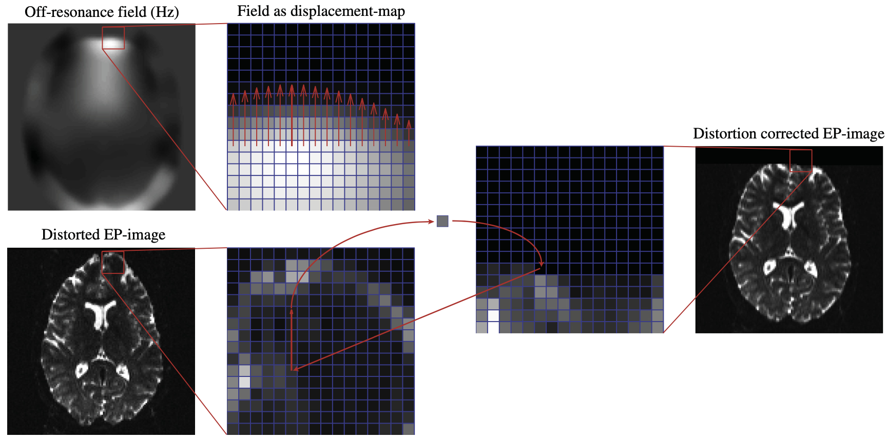
Unwarping an Image when the Off-Resonance Field is Known
如果off-resonance field 和 acquisition parameters 知道,那么就可以从distorted image 重建出corrected image。
-
Fieldmaps
-
How to Choose $\Delta TE$ for your Fieldmaps