Physical and numerical phantoms for the validation of brain microstructural MRI A cookbook
Numerical Phantoms for Structural Modeling
Laplace equation, finite difference method, finite element method to solve Bloch-Torrey equation
Diffusion
a potential mistake: $\theta=\pi v, \phi=2\pi u$。应该是$\cos(\theta)=1-2v,\phi=2\pi u$。因为前一种在random sampling的时候,更容易在z方向上
采样完后计算dMRI signal,$\phi=-\gamma\int g(t)r(t)dt, S(g)=<e^{i\phi}>$。
每一个采样都是对propagator的一个采样。由于运算量大,propagator is sampled in finite order cumulant (up to 2nd order/ 4th order)。
dMRI signals are sampled in a finite range of q-space, 用cumulant expansion表示
In monopolar diffusion gradient, the diffusivity can be estimated by the second order cumulants of the diffusion displacement.
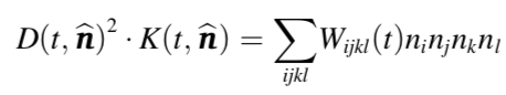
$D(t,\hat{n})=\frac{<(\Delta r \cdot \hat{n})^2>}{2t}, \Delta r=r(t)-r(0)$ 表示沿着$\hat{n}$的diffusion
the non-Gaussianity of the diffusion propagator can be evaluated via the (excess) diffusional kurtosis.
$K(t,\hat{n})=\frac{<(\Delta r \cdot \hat{n})^4>}{<(\Delta r \cdot \hat{n})^2>^2}-3$
diffusion tensor: fitting 3x3 tensor D to D(t,n) → $D(t,\hat{n})=\hat{n}^TD\hat{n}$
diffusion kurtosis tensor:
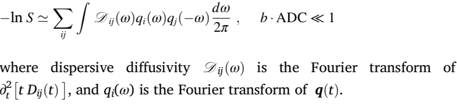
计算各种不同时间t下的$D_{ij}(t)$,从而计算 ADC with low b-value , based on Gaussian phase approximation
$ADC=-1/b\cdot ln(S)$
Susceptibility
根据磁化率公式可以计算$\Delta f(r)$,通过累加phase change $d\phi=2\pi \Delta f(r(t))dt$ 沿着particle diffusion trajectory r(t),the simulated signal of the echo time TE
$S(TE)=<exp(i\int^{TE}_0 d\phi)>$
How to set up a Monte Carlo Simulation
-
Designing the microstructure geometry
通过简单的2d/3d形状组合
restricted diffusion in intra-axonal space, the isolated pores has no influence on results,
hindered diffusion in extra-axonal space, results depend on packing geometry
WM axon 的结构一般是randomly packed geometry,但是直接生成随机的结构比较麻烦。collision-driven packing generation。
size of phantom geometry » diffusion length
-
Particle number
$error \propto 1/\sqrt{粒子数}$
一般来说需要粒子束 $>10^5$。
-
Step size
一般来说小于1/10的cylinder radius
step time $\delta t<\delta$ (gradient pulse width)
no standard, only sanity check
-
Step number
simulation一开始几千个step 产生的结果可能不准确,因为离散化造成的误差。通过检验diffusion kurtosis来指导step number。$K(t) \propto 1/N_{step}$
- Boundary condition (substrate edge)
- mirroring
- periodic boundary condition: 如果两侧边界microstructure 不连续,就可能有问题。
- Impermeable, permeable and absorbing membranes
- impermeable: 当作完全弹性碰撞
- permeable: 有一个$P_{EX}$的概率穿过membrane,有一个$1-P_{EX}$的概率reflection
从compartment 1 → compartment 2,particle 行进$\nu \cdot \delta x_1$,再同方向前进$(1-\nu)\delta \cdot x_2$,这一个step 产生的总共T2 weighting signal 是$e^{-\nu \cdot \delta t/T_2^{1}}e^{-(1-\nu) \cdot \delta t/T_2^{2}}$
- Particle-membrane interaction: elastic collision (specular reflection), diffuse reflection, and equal-step-length random leap
- elastic collision,反射后方向与入射方向相同
- diffuse reflect,反射后方向随机,反射前后总的step length 不变
- equal step random leap,不常用
-
Relieving the computational bottleneck
lookup table
How to Proof check your Monte Carlo Simulation Framework
- Free diffusion
-
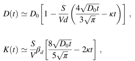
Diffusion time dependence in short-time limit (S/V limit)
simulation results中的D,K必须满足这两个条件
-
Analytical solutions for time-dependent diffusion
在最简单的有解析解的形状上试验
(parallel planes, cylinders and spheres with imper- meable (non-)absorbing membranes)
-
Particle density balance for the water exchange
average particle densities in each compartment remaining the same
Examples
Physical Phantoms to Validate Brain Microstructure
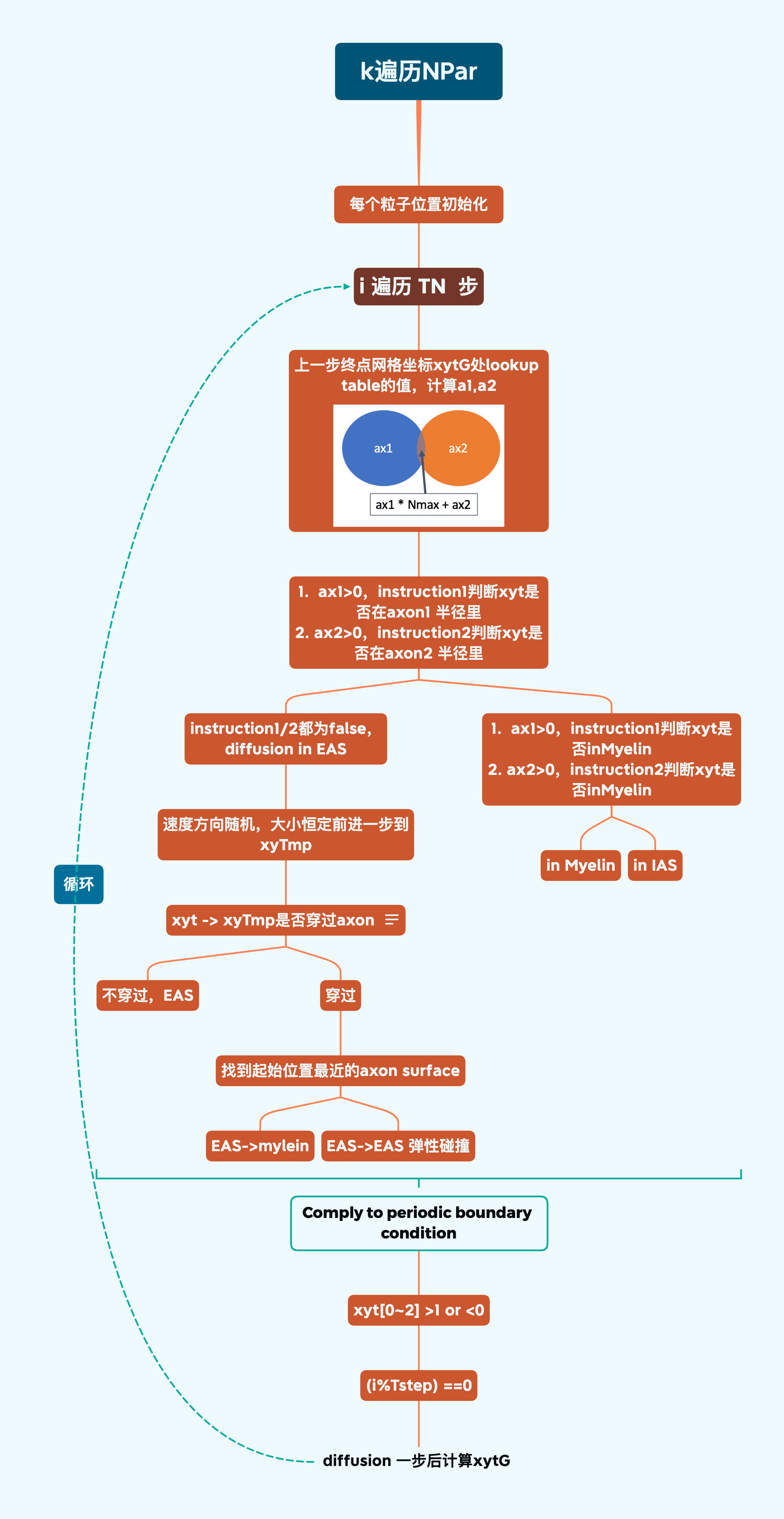
Fig.4 Simulation 2, How the code was implemented!